Causality, Generalization, and Reinforcement Learning
Oh my!
Reinforcement learning has a generalization problem.
To be more precise, RL has a lack of generalization problem. The RL objective is to maximize cumulative discounted reward in an environment, and over the years algorithms have gotten better and better at doing so in a variety of tasks. However, research has focused on maximizing returns in a single environment. This yields agents vulnerable to failure when the environment changes even slightly, and leaves the community in a position where we have more superhuman Atari-playing neural networks than we could possibly need, but (without training on thousands of environments) no agents that are robust to a change in the colour scheme of the game they were trained on.

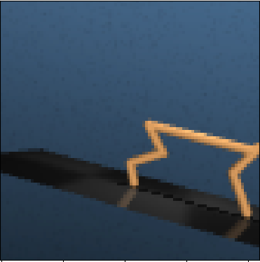
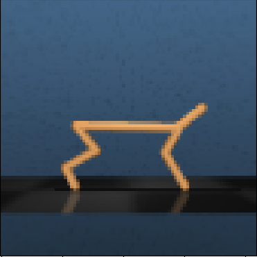
Can a mujoco agent trained on the first two observations generalize its knowledge of the laws of physics to the third image?
Our recent ICML paper proposes a way to address this problem. It’s impossible to train an agent to attain good performance under any possible new environment, so we’ll focus on generalization to new environments that are behaviourally equivalent, or bisimilar, to the training environments. For example, we’d like a Mujoco agent trained with pixel-valued observations from one or two camera angles to learn how to control a simulated robot, and to generalize what it learns to new camera angles. Standard RL methods have a really hard time doing this out of the box, unless you train on a massive number of camera angles. Our method, as we’ll see later, does quite well with only two training angles.
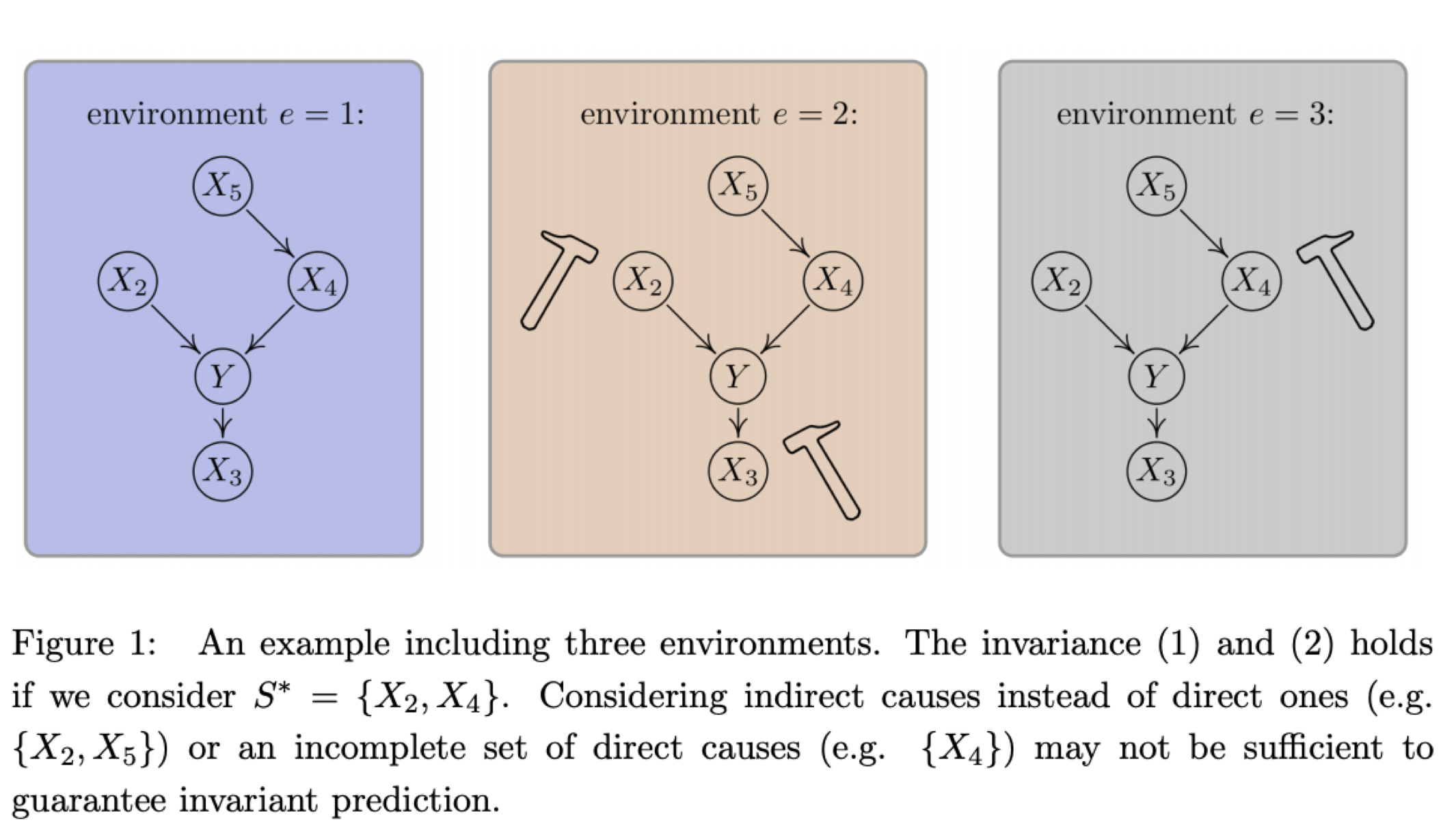
An illustration of the intuition behind Invariant Causal Prediction.
We do this by leveraging a tool from causal inference called Invariant Causal Prediction, or ICP. The key idea motivating this approach is that causal relationships between variables are invariant to changes in the environment, and so by picking up on relationships that exist across a number of training environments, the agent will be capturing the causal structure of the environment, which will help it generalize to new changes to the environment. We modify this approach to find causal parents of the return when training an RL agent on a collection of training environments with certain properties. We show that in some settings, the variables found by ICP correspond to a model irrelevance state abstraction (or MISA, which we’ll explain shortly).
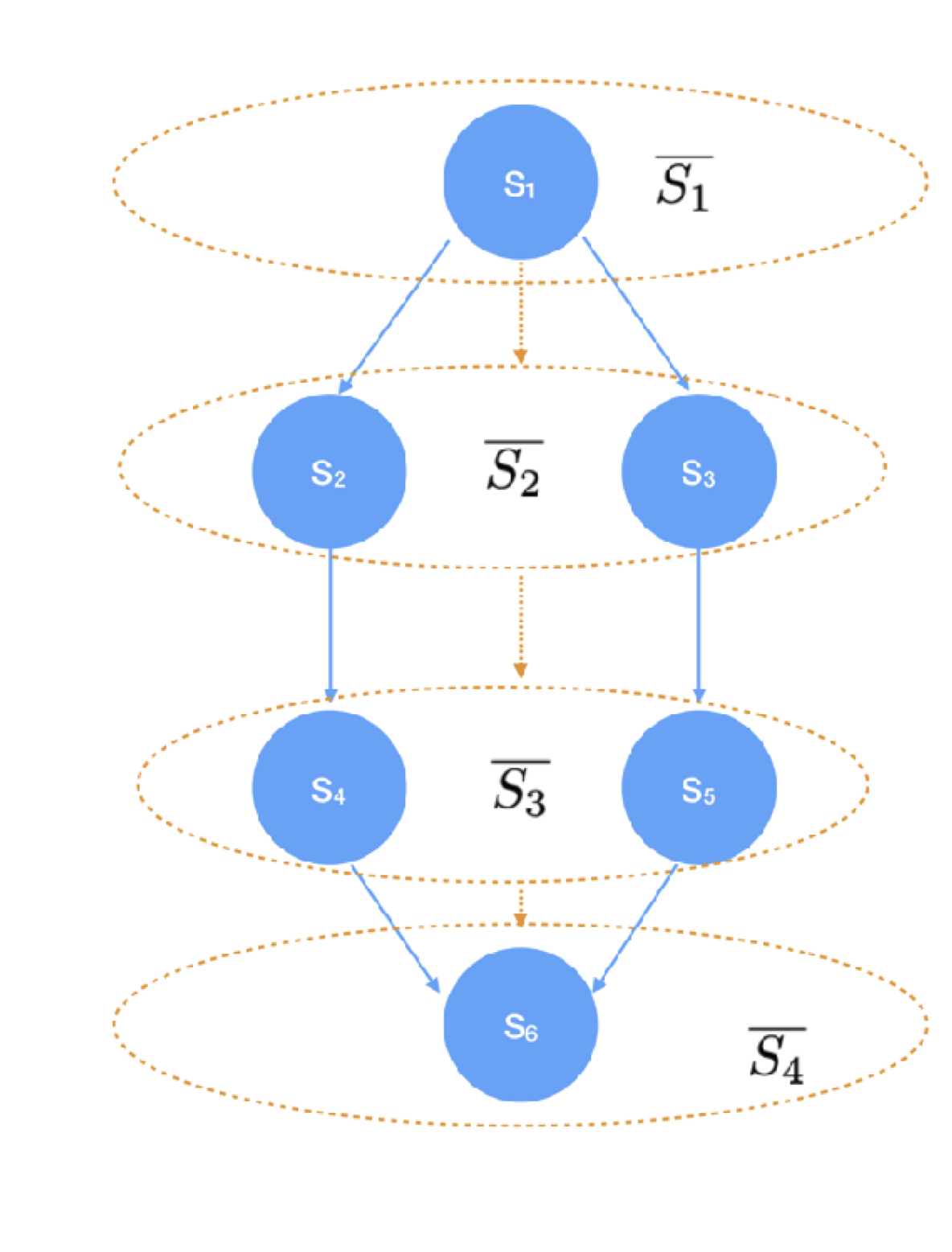
Orange line indicates abstract states.
A state abstraction \(\phi : \mathcal{S} \rightarrow \bar{\mathcal{S}}\) is a function that simplifies the state space of an MDP. For example, in the MDP on the right (we assume no reward for simplicity), the transition dynamics for each pair of adjacent states are equivalent, and so we can simplify our state space by equating these pairs without losing any important information. In order to be useful for planning, we need \(\phi\) to satisfy certain properties: it should only map two states together if they have the same reward, and the abstract state transition dynamics should be equivalent to the dynamics of the true MDP. A state abstraction satisfying these properties is a model irrelevance state abstraction.
Normally, model irrelevance refers to a single environment, but it’s pretty straightforward to extend this definition to multiple environments. To do so, we’ll assume that our environments correspond to different observation maps of a block MDP. The block MDP assumption states that observations and transitions are drawn from a simpler underlying state space: for example, an agent might observe many different angles of the same scene, but the different observations all correspond to the same positions of the objects, and so are in some sense equivalent. We’ll say that a state abstraction \(\phi\) over a family of MDPs \(\mathcal{M}_{\mathcal{E}} = \{\mathcal{M}_e | e \in \mathcal{E}\}\) is a model irrelevance state abstraction if it is a MISA for each individual environment. We’ll be particularly interested in finding minimal MISAs, where if \(o\) and \(o'\) are observations corresponding to the same underlying state in environments \(\mathcal{M}_e\) and \(\mathcal{M}_{e'}\), then \(\phi(o) = \phi(o')\).
We can visualize these families of MDPs as graphical models with the following diagram: the ‘true’ state is \(s_t\), which feeds in, alongside some environment specific noise \(\eta_t\), to produce the observation \(o_t\). We assume that the reward \(r_t\) only depends on \(s_t\). For example, we might imagine an agent whose state is an \((x,y)\) coordinate and whose goal is to travel to the line \(x=10\). Then the reward will only depend on the \(x\)-coordinate, and \(y\) will be a ‘spurious variable’, whose value can change between environments without affecting the reward or optimal policy. We could then assign \(x\) as \(s_t\), \(y\) as \(\eta_t\), and \(o_t = (s_t, \eta_t)\) to obtain the following graphical model.
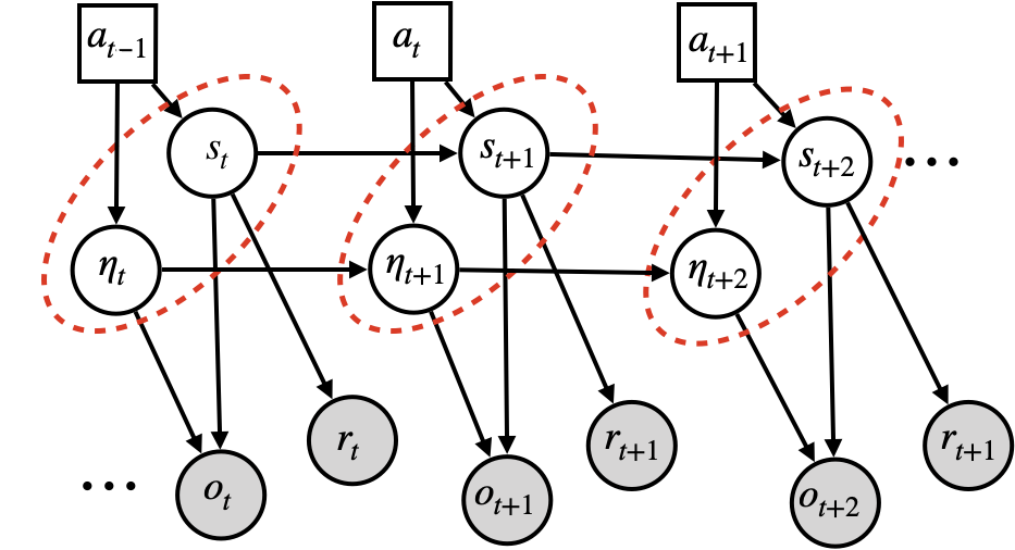
The first major insight of our paper is to show that in MDPs where the observation space is some collection of variables \((x_1, \dots, x_n)\) whose transition dynamics can be characterized by a causal graph \(\mathcal{G}\), the causal ancestors of the return in this graph correspond to a model irrelevance state abstraction. To prove this, we show that knowing the causal parents of the reward is sufficient to predict its expectation, and that more generally knowing all of the causal parents of any particular variable in the state abstraction is sufficient to capture its next-state distribution. Then since the set of causal ancestors of the reward is closed under taking parents, it follows immediiately that this set of variables will be sufficient to predict the next-step distribution of itself, and to predict the expected reward. This is precisely what it means to be a model-irrelevance state abstraction.
What’s really great about this state abstraction is that it’s going to be robust to changes in the variables that aren’t causally related to the return – this means that for any new environment with interventions to spurious variables, a reinforcement learning agent trained using this state abstraction won’t perform worse than on its training environments. This is a much nicer guarantee than what we’d normally get from applying a PAC-style bound on the generalization error of an agent, because it leverages the structure of the environment. We demonstrate this using a toy environment with an agent trained to predict the value of a policy using linear value function approximation. One agent is trained using a subset of the observation space that corresponds to this causal ancestor set. The other is trained on all of the variables. The causal state abstraction agent doesn’t see any degradatiion in performance when the spurious variable is intervened on. However, the agent trained on the whole state space sees monotonically increasing Bellman error as the intervention distribution on the spurious variable moves further and further from the training distribution.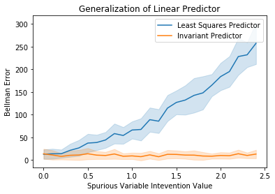
Comparison of Bellman policy evaluation error for causal and identity state abstractions under intervention on a spurious variable.
And there you have it folks. We’ve solved generalization to new environments in reinforcement learning. Thank you for your attention. Come back next time when we present our AGI.
Unfortunately, the structure we assume for the idealized setting is almost never present in interesting RL problems. Now we need to deal with the types of environments that give RL theorists nightmares: the rich observation setting with nonlinear function approximation (i.e. Deep RL). Causal inference can provide us with inspiration for this setting, but unfortunately we have to leave behind our provable guarantees and move into the land of approximations. Here there be Bellman errors.
We present a neural network architecture which aims to capture the invariant structure across training environments by learning an environment-invariant latent transition model, which is then used to construct a policy. The idea here is that if we learn how to predict the structure of the environment in a way that’s invariant across the training environments, then this should, fingers crossed, give us a state abstraction that will also capture the latent structure of new environments. Then the policiy we learn based on this state abstraction should generalize well to the new environments as well.
For this more complex setting, we provide some bounds on the error of continuous state embeddings that only approximately capture the underlying structure of the MDP in new environments. These bounds depend on the accuracy of the learned latent-space model on its training environments, and the distance between the new environment’s latent embedding and the training environments. These bounds depend on the embedding performing sensibly in the new environment, which is unfortunately not guaranteed by the method we propose for the rich observation setting, so we resort to empirical evaluations to see how it does.
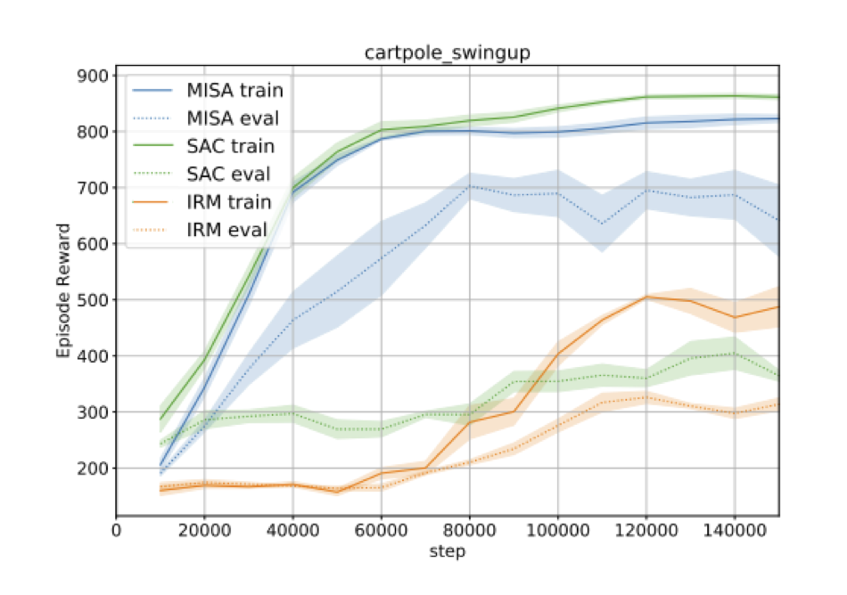
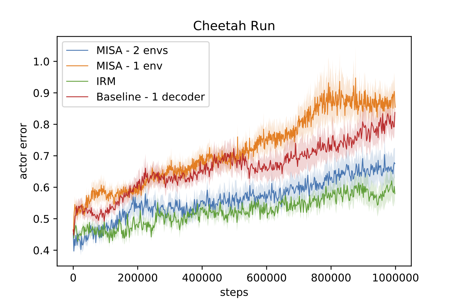
Comparison of our method with other baselines in the rich observation setting.
Fortunately, our method is able to pick up the invariant structure quite well in a number of tasks, outperforming the baselines that have the same architecture but don’t enforce invariance across the training environments. As another baseline we also compared against Invariant Risk Minimization (IRM), another method for learning invariant structures in the rich observation setting. We found IRM to be very sensitive to learning rate schedules and hyperparameters; in one task we found it outperformed our method, but in the RL task we evaluated it failed completely to solve the task even on the training environments.
While our paper definitely isn’t the last word on generalization in RL, I think it’s a good first step in leveraging invariance across environments to improve performance in new settings. We’ve shown that capturing causal structure in the environment is in some sense something that we’re already trying to capture in the state abstractions we want in RL. We’ve further demonstrated that incentivizing models to exhibit the right kind of invariance can help them to generalize well to new environments, whereas models trained without acknowledging the structure in the task they’re trained on will fail to do so or require enormous amounts of training data.