Auxiliary tasks in RL

##Introduction

One of the most fundamental problems in reinforcement learning (RL) is how to learn a good value function. We’ve gotten pretty good as a community at getting agents to learn good value functions for some domains, like Atari games or robot control simulators, but we still have a lot of room for improvement. There are hundreds if not thousands of papers coming out every year with new tricks to learn better value functions that let agents perform even better on these tasks.

Intuitively, you might think that the best way to figure out how good an action is would be to laser-focus on only the components of your input that tell you how much reward you’re going to receive in the future. If you’re learning how to play soccer for the first time, for example, you should pay attention to the ball. You don’t want to concurrently try to learn how to take a penalty kick and estimate the number of dandelions behind the net.

Estimating the number of dandelions behind the net is an example of what the RL community calls an auxiliary task. It’s not your main goal, but you’re still using it as a learning signal while you’re messing about trying to figure out how your environment works. Auxiliary tasks have been shown to significantly improve agent performance in reinforcement learning across a huge range of domains. Typically these tasks are chosen to be a bit more useful than counting dandelions on a soccer pitch: a better analogy might be learning to move the ball from one side of the pitch to the other, or learning to predict which direction a player will run. If you were dropped onto a soccer pitch with no concept of “hand ball”, “goal”, or “opposite team”, it would take a lot of random running about before you discovered that putting a ball into one of the nets gives you a point. Learning to control parts of the game will likely help you once you do figure out that putting a ball in the net earns you a point, since you don’t now need to learn how to kick the ball from scratch.

But how does trying to predict something other than your main objective help deep RL agents? The answer isn’t super clear. The general consensus in the community is learning with auxiliary tasks leads to better representations (outputs of intermediate layers of a neural network), although what makes a representation better seems to follow a circular definition of “it leads to improved performance”. This isn’t a super satisfying definition, so in our (joint work with Mark Rowland, Georg Ostrovski, and Will Dabney) recent paper, we tried to dig into what’s happening in agents’ representations that might be leading to performance gains.

##Learning Dynamics

We did this by analyzing an idealized model of representation learning. There are a lot of different value-learning algorithms in RL, but we’re going to focus our analysis on temporal difference learning in the policy evaluation setting (i.e. the agent is just trying to figure out the value \(V^\pi\) of a fixed action selection rule \(\pi\)). Even more specifically, we’re going to focus on TD(0) updates, which update the value function at time \(t\), \(V_t\), based on the observed reward and the expected value at the next state.

\[ V_{t+1}(x) = V_t(x) + \alpha( R^{\pi}(x) + \gamma \mathbb{E}_{x' \sim P^\pi{x'|x}} V_{t}(x') - V_t(x)) \]

In matrix notation, we write this update as follows, where \(V_{t}\) refers to the vector representation of the value function:

\[V_{t+1} = V_t + \alpha(R^{\pi} + \gamma P^\pi V_t - V_t) \]

We’re going to focus on the learning dynamics induced by this update rule. By learning dynamics, we’re referring to how the value function changes over time. We’re going to make a simplifying assumption and focus on continuous-time dynamics, where we model the discrete update described above as a continous time system whose time derivative looks as follows:

\[\begin{equation} \partial_t V_t = R + \gamma P^\pi V_t - V_t \end{equation}\]

We can visualize this system for a simple two-state MDP to get a sense of how the temporal difference updates compare to performing regression on the target value function \(V^\pi(x)\) directly.

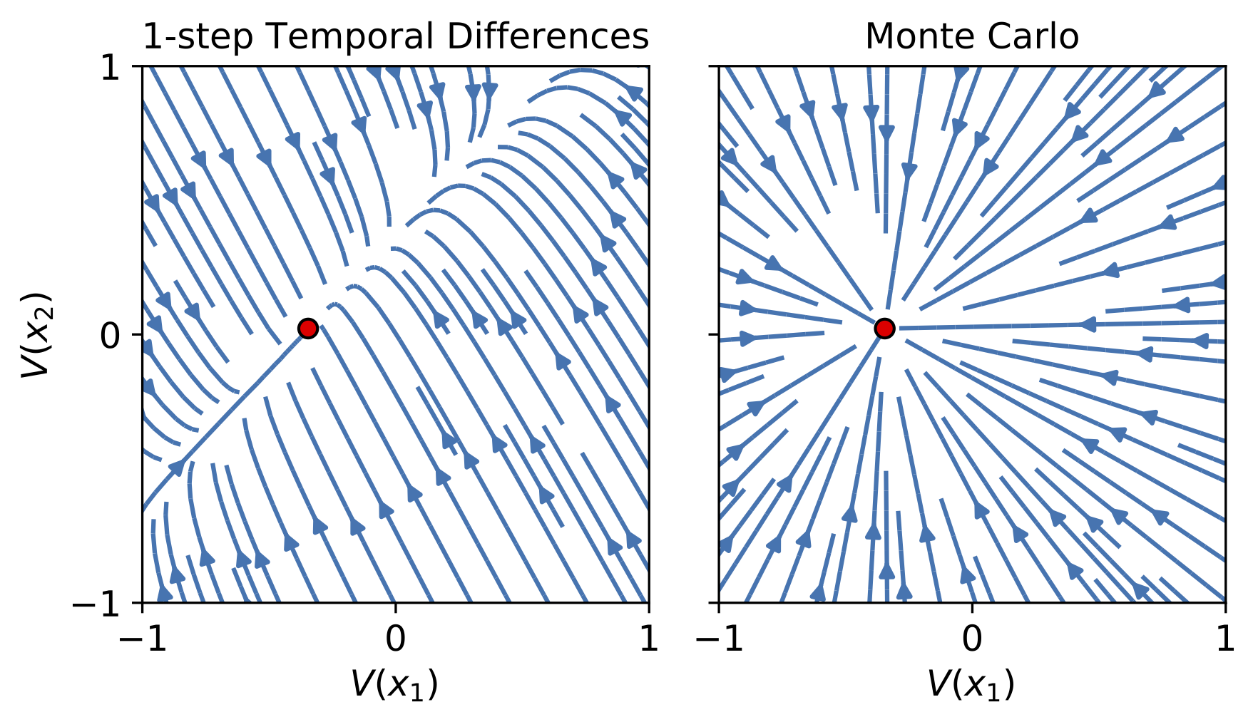
Evolution of randomly initialized value functions as they converge to \(V^\pi\) in a simple 2-state MDP, as shown in the paper this post is based on.

The lines in these figures show the path that a value function initialized at a point on that line will follow if it evolves according to the continuous time dynamics given by either Monte Carlo or TD updates. The MC updates follow a straight line to \(V^\pi\), which is exactly what you’d expect for a regression objective. The TD updates follow a more curved path, and converge along the line corresponding to the constant function \((\alpha, \alpha)\).

Why does this happen? Well, one thing to note is that for any 2x2 stochastic matrix \(P^\pi\), the constant function \((\alpha, \alpha)\) is an eigenvector of \(P^\pi\) with eigenvalue 1. In particular, it’s the eigenvector corresponding to the largest eigenvalue. So while the MC updates are going straight for \(V^\pi\), the TD updates are headed almost-straight for the top eigenvector of \(P^\pi\), and then once they’re close to that line they go straight to the target \(V^\pi\). In other words: they’re converging to a subspace determined by the top eigenvector of \(P^\pi\).

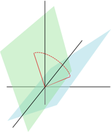
We used a generalized notion of the “angle’ between two subspaces to prove convergence. Figure by Mark Rowland.

In our paper, we formally show that under a specific measure of distance between subspaces (see the picture on the right), the “error term” \(V_t - V^\pi\) converges to the subspace spanned by the top eigenvectors of \(P^\pi\). When \(R^\pi=0\), the value function converges to zero along the subspace spanned by the top eigenvectors of the environment transition dynamics. Thus even when \(V^\pi = 0\), the learned value function is picking up some of the structure of the environment.

This is all well and good, but it doesn’t answer the question we originally posed: how do TD updates affect agents’ representations? For this we have to look at a different dynamical system.

Representations

We’re going to assume an agent’s value function can be broken down into two parts: a feature map \(\phi\) which takes observations \(x\) as input and outputs a vector \(\phi(x)\), and a linear value approximator \(w\). The value function of a state \(x\) can then be given by \(V(x) = \langle \phi(x), w \rangle\). This simulates the penultimate layer of a neural network feeding into a linear map to produce the output.

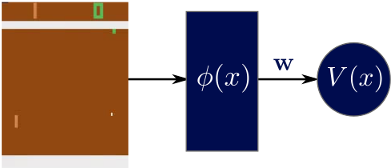
Our representation learning model.

Temporal difference updates for linear function approximation follow a semi-gradient with respect to the TD prediction error. We say this is a semi-gradient because we’re trying to move the predictions closer to the targets, not move the targets closer to the predictions (this would be a bit like if you start your drive to work, estimate it will take you 30 minutes, then see an accident on the road that will make you 15 minutes late and instead of updating your original prediction to account for the traffic jam you decide that traffic jams don’t slow you down).

\[ \partial_t w_t = \sum_{x \in \mathcal{X}} (r(x) + \gamma \mathbb{E}[V_t(x')] - V_t)\nabla_w V_t = \Phi_t^\top (R^\pi + \gamma P^\pi \Phi_t w_t - \Phi_t w_t)\]

Where similarly to how \(V\) is the vector of values for each state, \(\Phi\) is the matrix whose rows are feature vectors.

Because we’re interested in feature learning, we’ll also model how \(\phi(x)\) changes as a function of time. We’re going to make the assumption that \(\phi(x)\) changes exactly according to the gradient updates. In practice, \(\phi\) is parameterized by the weights of a neural network, and updates with respect to the weights may lead to changes in \(\phi\) that are different from the gradient computation we do here. However, this setting still tells us what really really big neural network are “trying” to do.

\[\partial_t \Phi_t = (R^\pi + \gamma P^\pi \Phi_t w_t - \Phi_t w_t) w_t^\top\]

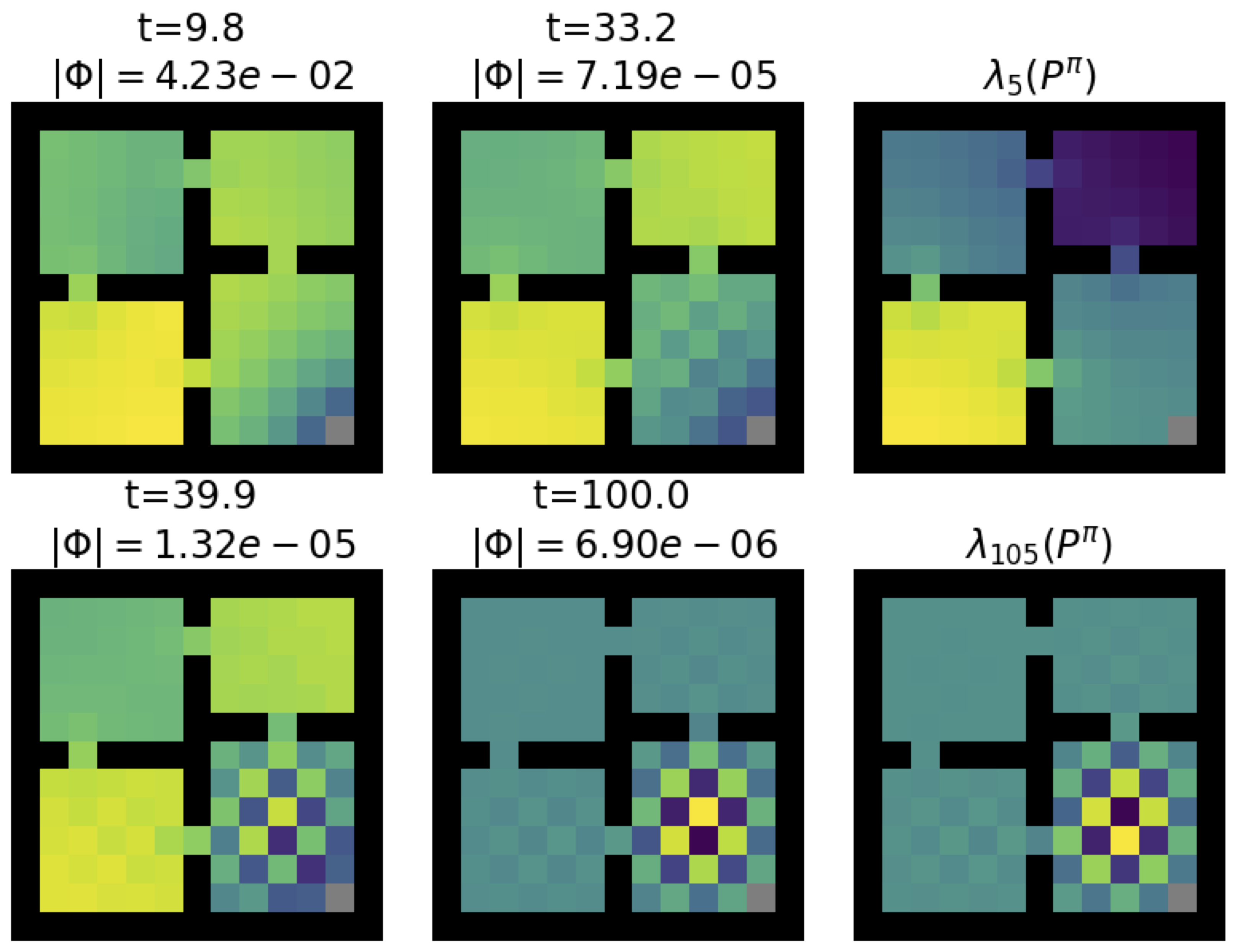
Evolution of features during training.

Because \(\Phi_t\) and \(w_t\) depend on each other, this system of equations evolves in hard-to-predict ways and so we can’t necessarily obtain a closed-form solution. We ran some simulations and found that the features did seem to end up looking like different eigenvectors of the transition matrix, but there wasn’t a straightforward pattern in which eigenvectors they ended up resembling. However, we are able to show that similarly to how the value function can be shown to pick up information about the environment transition dynamics, so too can the representation \(\Phi\). This leads to the main take-away of the paper.

Under some assumptions on \(w_tw_t^\top\), the representation \(\Phi_t\) converges to the subspace spanned by the top eigenvectors of \(P^\pi\).

The assumptions here are relatively technical, so I won’t get into them except to say that under some auxiliary tasks with fixed or slowly updated weight vectors, these assumptions end up being satisfied. We are then able to get the closed-form feature trajectories for a range of auxiliary tasks where the agent is being trained to predict many (OK, we take a limit of infinitely many) things.

One particularly interesting setting is random cumulant prediction, where we predict the value corresponding to a randomly generated reward function. Under this auxiliary task, we find that the features \(\Phi_t\) converge not to zero, but to a random subspace which is biased towards the top singular vectors of the resolvent matrix \((I - \gamma P^\pi)^{-1}\). In other words: under random cumulant auxiliary tasks, not only does the representation pick up information about the environment dynamics, but it also doesn’t collapse to zero!

Results

Based on the above observations, we hypothesize that predicting the value of random rewards should be a useful auxiliary tasks for settings where the agent doesn’t see rewards until relatively late in training – the sparse reward setting. The idea here is basically that under the value prediction objective and auxiliary tasks that use the observed extrinsic reward, the agent’s predictions and features will collapse to be effectively zero because the target value function is zero. In contrast, a random cumulant agent will avoid representation collapse and while still picking up useful information about the environment structure. Indeed, this is what we see: predicting many random things isn’t particularly helpful when the environment reward is giving you a good learning signal, but when you aren’t receiving reward it can help keep you from concluding that everything is equally terrible so that when you do finally see rewards you are able to use them to improve your value function.

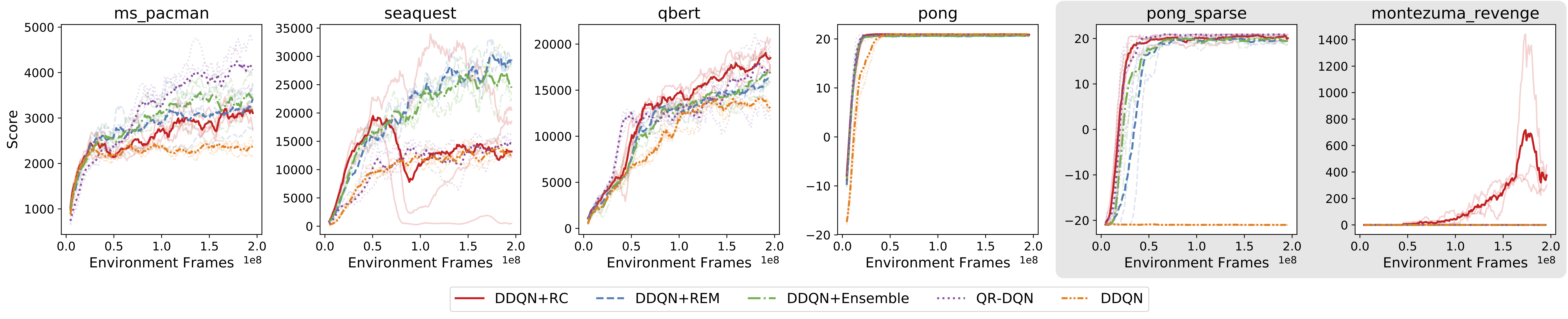
Atari results. DDQN+RC is the agent trained with the random cumulant auxiliary task. All other agents use the observed environment reward to perform updates. DDQN+RC is the only agent to attain nontrivial reward in Montezuma’s Revenge, a hard exploration task in Atari.

So what can we conclude from this? There are two main take-aways: first, value functions and representations trained with TD updates pick up information about the transition structure of the environment. Second, auxiliary prediction tasks can be useful to ground the representation in sparse reward environments to prevent the agent from mapping all states to the zero vector. While this paper is hardly the final word on representation learning in RL, I think it provides some neat insights into how learning algorithms and representations interact that might prove useful for the community.