Do we know why deep learning generalizes yet?
It depends on your epistemology.
Deep learning has seen tremendous empirical success in recent years. However, theoretical understanding of deep neural networks remains limited.
You can find these two sentences, and variations thereupon, in probably hundreds of papers that try to prove things about deep neural networks (or, if you’re like me, prove things about linear models, then close your eyes and say “in the limit of infinite width” to yourself until you can sleep at night). I for one have been guilty of using variations on these two sentences in the introductions of many paper drafts and course projects – with good reason. The statement above is strictly speaking true: deep learning has been absurdly successful at a diverse range of tasks, and we definitely have a lot of unanswered questions about why exactly this success is happening. I would say that the second sentence in particular was probably a fair take in 2015. At the same time, there have been a lot of papers over the past seven years trying to develop a theory of deep learning. Is it still fair to say that we don’t really understand deep neural networks?
In this blog post I’m going to attempt to answer this question, and in the process figure out whether the introduction to every paper I tried to write in the first year of my PhD was a bald-faced lie. Most of the community’s confusion about machine learning stems from its successful generalization performance, so throughout most of this blog post I’ll use “understanding deep learning” and “understanding why deep learning generalizes” interchangeably. To make the question more tractable, I’ll break up the topic of ‘understanding deep learning’ into three components:
Interpolation: do we know why giant models that perfectly fit their training data so often also perform near-optimally on test data?
Optimization: why does gradient descent on a massively over-parameterized nonlinear function space 1) converge 2) to solutions with a relatively small generalization gap?
Architecture design: do we understand why the community’s favourite architectures are so successful?
Historical background
Before diving into recent work, it’s helpful to understand the origins of the study of generalization. Strictly speaking, analysis of the convergence rates of various statistical estimators dates back to the nineteenth century. Supposing, for example, that your goal is to estimate the mean of a probability distribution from samples, you can use the standard empirical mean estimator: \[ \widehat{\mu}(x_1, \dots, x_n) = \frac{1}{n} \sum x_i \] and the expected error of your estimator can be characterized by its variance, which decays with the inverse of the number of samples. Of course, if what you care about is to minimize the “typical” error of your estimator, there are more complicated estimators that will do the job better – see e.g. Gabor Lugosi’s NeurIPS 2021 tutorial.
In machine learning problems we’re usually interested in a more complex statistic of the training data than its empirical mean. For example, we may want to estimate the classification error of a hyperplane that separates a set of inputs according to their labels. Of course, the hyperplane we are most interested in is the one which best separates our finite dataset, but the error of the best-fit hyperplane on a set of points will be lower than its expected error on other points drawn from the distribution, so we cannot straightforwardly reuse the training dataset to estimate the expected error. This makes bounding the error of this estimator more challenging, and necessitates more complex mathematical tools: these are what we now call generalization bounds. The first paper I’m aware of to produce something that a modern reader would call a generalization bound was due to Vapnik in the late 1960s, with the engrossing title On the Uniform Convergence of Relative Frequencies of Events to Their Probabilities.
The key takeaway from this paper is that by restricting the expressivity of a class of function approximators \(F\), one can guarantee that the training loss of the function that best fits the training data will converge to the expected loss of the best-fit approximator over the entire distribution. This represents a worst-case bound, because it says that the probability of drawing a particularly unrepresentative sample such that there exists some function in \(F\) that can obtain an extremely low loss on this set while performing poorly in expectation over new samples is low. In other words, the odds that you sample a training set for which there is a terrible empirical risk minimizer is low. This result is incredibly pessimistic: it says that even if there are a million functions in \(F\) that fit the training set and also get a low expected loss, if even one function in \(F\) has a large expected risk on new samples then your bound will depend on that one.
Obviously, this kind of guarantee is terrible for explaining generalization in large neural networks because- DNNs are universal function approximators, which means that there will often exist parameters that can interpolate the training set but obtain arbitrarily bad performance on new data, and
- the way we train DNNs (see the section on convergence) means that we’re extremely unlikely to find these misleading parameters.
To understand generalization in neural networks, we need to understand how the architectures and training procedures used in practice bias the search algorithm towards ‘good’ parameters. A really smart uniform convergence bound might have some success with this, but it will have to do a very good job of restricting the function class \(F\) to reflect this bias, and potentially also take into account the ‘niceness’ of real-world datasets. This seems hard to do analytically, but if there’s a paper on arxiv tomorrow that gives a formula for this inductive bias I will be pleasantly surprised.
It’s also unclear whether generalization bounds are necessarily the right tool for providing any explanation of deep learning’s generalization performance in the first place. A generalization bound is a mathematical truth about a learning algorithm applied to a function class. It doesn’t make falsifiable predictions: it is either true or false, and it is verified by the correctness of the corresponding proof, not by attempts to falsify its predictions experimentally (although it’s possible to shoehorn the rankings of bounds into a predictive theory and test that, in which case most bounds tend not to fare particularly well). In this sense a generalization bound is very different from a scientific theory that tries to explain an empirical phenomenon. Because this blog post is about understanding and explaining the empirical generalization performance DNNs, I will mostly omit prior work computing generalization bounds except where these bounds are actually correlated with ‘real-world’ generalization – which, as Dziugaite et al. show, is quite rare.Interpolation
A really exciting line of work over the past few years has studied the properties of interpolating predictors: learning algorithms and model classes that can attain zero loss on the training set. This is the regime that most DNN architectures tend to fall into. Large neural networks are incredibly expressive, and the ability of DNNs to interpolate even completely random labels of their training data has been well-studied. One intriguing finding in this regime is the double descent phenomenon, which has been observed in linear models, in kernel learning, and in deep neural networks.
Double descent & benign overfitting
The double (or indeed multiple) descent phenomenon shows that as a model becomes increasingly over-parameterized, it can obtain increasingly better generalization performance long after it has reached the threshold needed for interpolation. Rather than increasing the risk of overfitting, adding more parameters to a model can in many cases shrink the generalization gap, resulting in functions which interpolate their training data and exhibit reasonable behaviour on the support of the data-generating distribution. Of course, the way that you add these additional parameters is crucial to ensure that the double descent behaviour occurs.
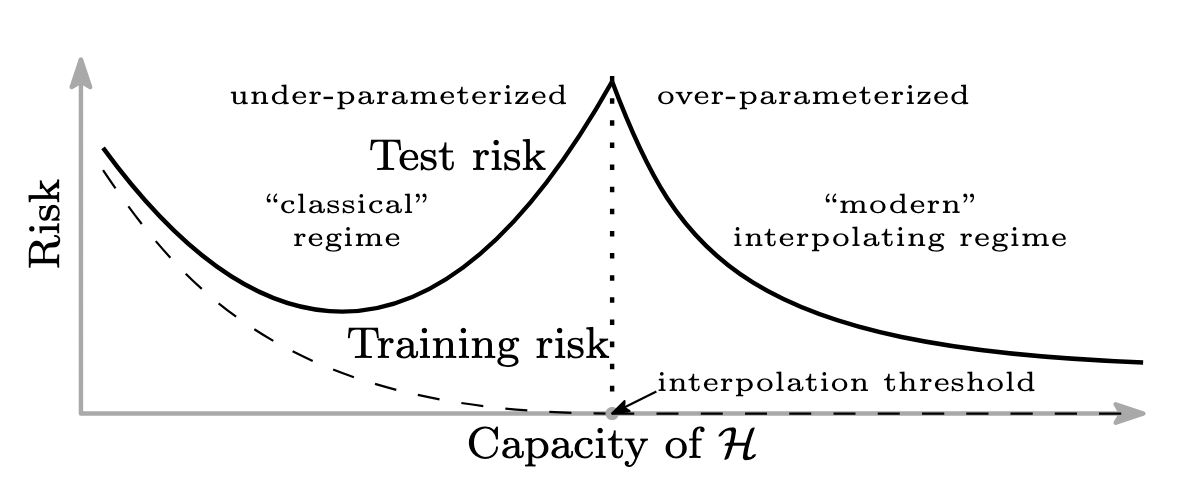
A double descent curve characterizing generalization error as a function of model capacity in neural networks (Nakkiran et al.)
Peter Bartlett has been giving talks since before I started my PhD on the second descent region of these double descent curves, where the function approximator falls into the regime of benign overfitting. This describes the situation where the predictor has overfit in the sense that it attains zero loss on a noisy training set, where the true optimal predictor over the whole distribution would attain non-zero loss, but nonetheless attains an expected risk close to that of the optimal predictor. In other words, attaining a lower-than-optimal loss on the training set doesn’t hurt its ability to generalize near-optimally. A recent paper studying benign overfitting in linear models gives some intuition on when we can expect this to occur as a function of the spectrum of the feature covariance matrix. The key idea is that most of the mass of the feature-generating distribution needs to reside in a small number of dimensions relative to the size of the training set (in order to accurately estimate the parameers of the linear model), but also be diffuse enough that the label noise in the training set doesn’t completely overpower the signal from the features (to avoid pathological overfitting). While it’s unclear how much this intuition carries over to neural networks, where the features of the input are learned, the idea that the training set needs to be big enough to capture the modes of the data distribution, but that the noise in this dataset shouldn’t carry undue influence over the learned parameters, is plausible.
Increasing over-parameterization can also increase the smoothness/robustness of the learned function, as an exciting Neurips paper showed last year. This work, and others like it, observes that a sufficiently expressive function approximator will have an easier time interpolating its training data with a smooth function than a less-overparameterized model. This leads to a divergence from pessimistic generalization bounds, which take a pessimistic view over the larger function class and give looser upper bounds. In essence, in many classes of function approximators including neural networks, increasing the size of the function class via increasing the number of parameters results in functions that both fit the training data and are smooth, e.g. have a small Lipschitz constant relative to those found in smaller function classes. In other words, even though the worst functions in the class defined by wider networks might be worse, the best functions are better.
What this paper and others show is that there are many function classes, not just deep neural networks, for which a predictor can ‘overfit’ (in the sense that its empirical risk will be lower than its true risk) and still attain near-optimal generalization performance. This line of investigation is quite orthogonal to that of the uniform convergence bounds we will discuss next, in that it is in a sense more optimistic: many papers studying benign overfitting focus on the existence of good functions in a function class, rather than the existence of pathological ones.
Aside: the state of uniform convergence in DNNs
A flurry of recent papers have debated the very utility of generalization bounds as described above. The past ten years have seen a zoo of generalization bounds proposed to predict generalization in DNNs; these all have a similar flavour as the early uniform convergence results of Vapnik. Essentially, such a uniform convergence result is a statement of the following form: for any hypothesis set \(F\), with probability \(1-\delta\) over the sampled training set \(\mathcal{D}^n\), the error of the function \(f\) output by some learning algorithm \(\mathcal{A}\) given \(F\) and \(\mathcal{D}^n\) will be bounded by some function of the complexity of the hypothesis class, the number of samples, and \(\delta\). The distinguishing factor between such bounds arises in the notion of complexity used. Prior works have set this to depend on <a href=““https://arxiv.org/abs/1506.02617>various norms of the weights, distance from initialization, number of training steps, and the flatness of the local minimum.
Two notable recent works complicate this picture. First, Jiang et al. in their whimsically named paper “Fantastic Generalization Measures and Where to Find Them” observed that many of the complexity measures that appeared in generalization bounds for DNNs are actually negatively correlated with a model’s generalization gap. Historically, vacuous generalization bounds were excused by the argument that even if such bounds were a bit flabby, they still gave an interesting directional indicator of the relative performance of different models. A model with a lower upper bound, it could be argued, should be preferred over a model with a greater upper bound on its test error. However, empirical results suggest that many uniform convergence results for DNNs are not only vacuous but also useless as even directional predictors of generalization.
Second, Nagarajan et al. constructed a simple example showing that uniform convergence guarantees are fundamentally incapable of describing the generalization performance of some overparameterized model classes. The driving intuition behind these examples is to construct a high-dimensional input space and hypothesis class (whose size depends on the number of samples \(n\)), such that any predictor obtained by GD which attains near-zero risk will still misclassify some non-zero subset of the input space whose probability under the data-generating distribution is at least \(\delta\) – i.e., for any hypothesis the probability of sampling a dataset on which its empirical risk differs from its true risk by a large amount is at least \(\delta\). This frequency of so-called ‘bad’ datasets necessarily increases the value of any uniform convergence guarantee. While two recent papers have shown that modified analysis incorporating an auxiliary function class can avoid this pathology, I personally am still somewhat pessimistic about uniform convergence results ever explaining generalization in DNNs for any reasonable interpretation of generalization. The amount of pessimism necessary to obtain general guarantees forces the theorist to ignore a lot of the data-dependent properties that likely drive the strong generalization performance of neural networks.
Optimization
OK, so we’ve concluded that although we clearly have a better sense of why overparameterization isn’t the devil that classical generalization bounds initially made it out to be, we still don’t have a great sense of how the search process defined by gradient descent so often finds nice parameterizations that generalize fairly well. In fact, this observation consists of two somewhat independent miracles: first, we have no reason to expect a priori that GD on functions parameterized as neural networks should even find parameters that fit the training data. Second, even assuming we found these parameters, it’s not obvious that parameters that fit the training data should also perform well on the underlying distribution.
The difficulties of depth
Solving the first point was a major focus of research in the 1990s through to the mid-2010s. Initial implementations of neural networks were incredibly difficult to train, particularly in the “end-to-end” framework so popular today. For example, this classic paper provides a nice overview of the steps involved in training a digit classifier end-to-end back when this type of thing was new and exciting. In more complex vision tasks involving images of exotic objects like trucks and horses, however, one-shot training a neural network was pretty much impossible. Instead, people tended to pre-train features using supervised learning, and then fine-tune on the target dataset.
Getting large neural networks to work required solving two big technical problems. The first was one of raw computational power: training a big neural network requires performing a large number of arithmetic operations in parallel. For smaller MLPs, Moore’s law and patience were enough to get sufficient computational power to train the model using sequential operations. However, bigger networks saw a massive benefit from the discovery that GPUs, which are very good at doing parallel arithmetic operations such as matrix multiplication, could be used to train really big neural networks at lightning speed. This was what drove the huge improvement in AlexNet when it ‘solved’ ImageNet back in the early 2010s.
The second technical problem involved stabilizing neural network training to enable deeper network architectures. One major breakthrough in this regard came from finding nice initialization distributions so that gradients didn’t explode or vanish as they were propagated forwards and backwards through a network. One of the most popular initialization schemes used today, He initialization, aims for the following property: \[ \frac{1}{2}n_l \mathrm{Var}[w_l] = 1 \; \forall l. \]
The intuition behind why this property is desirable is straightforward, but I think it says a lot about how other tricks for deep learning have developed: essentially, try to get the gradients and activations in each layer to look like a Gaussian with unit variance. Similar intuition lies behind the Glorot initialization, which is almost identical to He but uses a uniform as opposed to Gaussian distribution to initialize the weights and a slightly different constant scaling factor. Batch normalization can also be interpreted as a means of keeping activations (and by extension gradients) roughly looking like unit variance independent gaussians. While I’m not aware of a particularly satisfying explanation of the effect of batchnorm layers, I and most other people I know share the intuition that a) poorly conditioned gradients (such as those you would get from highly correlated activations) are not friendly to optimization, and b) forcing activations to preserve the unit norm property throughout training as opposed to just at initialization is probably also beneficial for avoiding vanishing or exploding gradients.
Traversing the loss landscape
One interesting observation of the OG resnet paper is that back in the olden days of deep learning adding more layers to a network hurt accuracy not by causing overfitting, which is what I would have expected, but by kneecapping optimization dynamics so badly that the network couldn’t even converge to a reasonable training loss in the first place. Tricks like residual connections smoooth out the loss landscape enough that optimization can proceed in a relatively stable manner, in a way that’s relatively robust to the dimensionality of the search problem. Finding architectures that scale well to billions or trillions of parameters has played a huge role in enabling the impressive feats performed by giant pretrained transformers over the past few years.

Artistic rendering of an AI navigating the loss landscape via gradient descent. (DALL-E, 2022.)
Ultimately, training a neural network requires walking a very fine line between chaos and stagnation. With small learning rates and suitable initialization schemes, we find ourselves in the NTK regime, where optimization follows a nice convex geometry but the network is unable to do meaningful feature learning; larger learning rates and different initialization schemes lose the convexity guarantee but enable more interesting behaviour in the hidden layers of the network. Recent work analyzes how different initialization schemes can lead to the presence or absence of feature learning in the infinite-width limit of neural networks trained with gradient descent. And yet it’s clear that there are also exciting properties of gradient descent on finite-width neural networks that still need to be explained: the existence of “lottery tickets”, the linear connectivity of local minima, and the tendency of SGD to learn functions of increasing complexity. Theoretical analysis has also characterized the bias of (stochastic) gradient descent towards flat minima, providing some intuition towards why gradient descent should prefer minima that generalize well – assuming it can find them in the first place.
Architecture design
The final piece of the puzzle is how the structure of neural network architectures biases gradient-based optimization towards minima that generalize well. As we mentioned in the previous section, gradient descent on any parameterized function class will prefer solutions that are flatter with respect to the loss. However, neural networks seem to have a particularly friendly inductive bias for a lot of natural datasets, beyond that which we would expect from a a preference for smooth functions. In some cases, the inductive bias is obvious: convolutional neural networks explicitly make it easy to learn functions that depend mostly on local structure, and which are relatively invariant to translations. This type of structure is clearly helpful for images, but it’s also relevant to a lot of other data types such as strings and even audio, where events that are close togehter in time are likely to be related. Similarly, neural networks that build in equivariance or invariance to group transformations will naturally have a nice inductive bias for learning functions that also exhibit these structures.
Some inductive biases, however, are a bit trickier to characterize. For example, many analyses have shown that neural networks trained with SGD are biased towards smooth functions. Other work has shown that the mapping from parameters to functions in DNNs is biased towards simple (with respect to an information-theoretic notion of simplicity) functions. One approach to study the inductive bias of neural networks is through the spectrum of the neural tangent kernel corresponding to the infinite-width limit of a given architecture, or to study the class of solutions obained by idealized neural network models on synthetic datasets. For example, a recent ICLR paper showed that ReLU networks converge to a combination of max-margin predictors.
Some other ways of measuring the utility of an inductive bias stem from using linear probes of randomly initialized (or in some cases pre-trained) feature maps. It has long been known that even randomly initialized convolutional networks provide features rich enough to obtain reasonable performance on image classification tasks. While the inductive bias of transformers is harder to get a handle on (though some recent work has made an impressive effort to do so), giant transformers trained on massive datasets presumably see enough of the world to encode a suitable “inductive bias” into their parameters, if not into the architecture itself. In fact, some interesting work has shown that fine-tuned CLiP models actually do better than more traditional conv nets at generalizing to certain classes of distribution shift – for example, they tend to generalize better between CIFAR-10 and CIFAR-10.1 compared to models trained only on CIFAR-10. Other work has identified specific sub-networks in transformer models that can perform tasks like induction, a phenomenon that might provide some intuition for phenomena such as the creatively named ‘grokking’, whereby networks can see sudden phase transitions in their generalization performance over the course of training even after attaining a low loss.
Conclusion
It would be a poor show for me to answer the titular question of this blog post with an equivocal answer like “it depends”. At the same time, the question of whether we understand generalization in deep learning is sufficiently vague that any pure yes or no answer would be incorrect. As a compromise I will try to enumerate a few sub-questions to which I’m confident I can give a binary answer.
“Given a neural network architecture with some set of parameters and some train set loss, can we accurately predict how well the network will generalize to data drawn from the same distribution as the training set?”“Do we know of properties of a neural network that correlate with generalization?”
“Have we identified quantities that are causally related to generalization?”
“Do we know of mechanisms by which gradient descent tends to pick out parameters that generalize better than the worst case ones?”
“Does the community have an intuitive understanding of why uniform convergence bounds tend to be uninformative in deep neural networks?”
“Do we understand how architectural choices influence generalization?”