When do adaptive optimizers fail to generalize?

There are many reasons to use an adaptive optimizer in machine learning, such as simpler hyperparameter tuning and faster convergence, but improved generalization is usually not one of them. While there have been mixed empirical results concerning whether adam or sgd tends to find solutions that generalize better in deep neural networks, the overall theoretical consensus seems to be that adam is prone to larger generalization gaps than gradient descent. But why should adaptive learning rates lead to solutions that generalize worse? As it turns out, it’s quite easy to construct a simple learning problem where gradient descent finds a solution that generalizes better than adam. This example should provide some intuition about the failure modes of adaptive learning rates and how they might arise in more interesting problems.

The regime of interest is simple: we consider a linear regression problem of \(n\) data points \(\boldsymbol{x}_i \in \mathbb{R}^{n+1}\). Letting \(e_i\) denote the \(i^{th}\) basis vector, we define each data point \(\boldsymbol{x}_i, i=1\dots n\) as \(e_i + y_i e_{n+1}\), where \(y_i \sim \mathcal{N}(0, 1)\). We set regression targets equal to \(y_i\), and look for a set of weights \(w\) such that \(\langle w, \boldsymbol{x}_i \rangle = y_i \; \forall i\). This is an over-parameterized linear regression problem, and so there are infinitely many solutions. These solutions have the interpretation of being some combination of two archetype solutions: the first is what I’ll call the ‘generalizing’ solution, and is of the form \(w_G = (0, \dots, 0, 1)\). The second is the ‘memorizing’ solution \(w_M\) and has the form \(\frac{1}{y_1}, \dots, \frac{1}{y_n}, 0\).

This problem is constructed to clearly distinguish between features that generalize between data points and features which `memorize’, and only contain data relevant to the data point where they are active. Here the feature \(e_{n+1}\) is constructed to contain all of the generalizable information between datapoints. While it doesn’t necessarily make sense to imagine how \(w_G\) will generalize to new data, we note that for a subset \(S = \{x_{i_1}, \dots, x_{i_k}\} \subset \boldsymbol{X}\), the induced memorizing solution \(w_M^S = \sum_{i_k} \frac{1}{y_{i_k}} e_{i_k}\) would obtain generalization error equal to \[\sum_{y_i \in S^C} y_i^2 \] on the remaining data points.

So what happens when we run gradient descent on this problem? For simplicity, we consider full-batch gradient descent with fixed step-size \(\alpha\). In this case, ignoring the negligible feature noise, we get \[\nabla_w \frac{1}{2} \|\boldsymbol{X}w - y\|^2 = X^\top(\boldsymbol{X}w - y)\] when \(w=0\), this becomes \[\nabla_w \frac{1}{2} \|\boldsymbol{X}w - y\|^2 = (y_1, \dots, y_n, \sum_{i=1}^n y_i^2)\]

If \(y_i\) is very small, then it is possible that \(\sum_{i=1}^n y_i^2\) can in principle be smaller than \(y_i\), however if we assume that the features are reasonably balanced, then in most cases the update to coefficient \(n+1\) will be much larger than the updates to the other coefficients. Intuitively, this is because there are \(n\) data points which are all contributing mass to this dimension, whereas each other dimension is only influenced by a single data point. A similar line of argument applies to future gradient steps, and the end result is that gradient descent will tend to bias towards solutions which are more similar to \(w_G\) than \(w_M\). Here’s the result I got by running gradient descent on the problem described above.

.

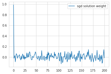
Now consider adam.

To simplify our job, we’ll actually consider RMSProp, as adam has a number of bells and whistles that would just distract us from our main object of interest: the adaptive step size. RMSProp is a batched version of a sign gradient method, where the idea is to perform an equal-sized update on all parameters, independent of the magnitude of the gradient associated with each one. For example, if \(w_1\) has a gradient of \(5\) and \(w_2\) has a gradient of \(0.001\), they both get the same update of \(\alpha\). This has some intuitive justification: if the gradient is small then you need to take a larger step to have a similar effect on the loss as if the gradient were large. Because we usually work with estimates of the gradient taken on minibatches, methods like RMSProp keep track of a running estimate of the gradient magnitude, and scale updates by this estimate to get a batched version of the uniform-update rule. For more details, see e.g. Geoff Hinton’s notes. If you do read through these notes, you might notice that while there does now exist some theoretical analysis showing that this type of method can converge, this analysis was decidedly not the motivating factor in the design of the algorithm.

Adam and RMSProp keep track of two quantities: a running gradient average \(\widehat{g}_t\), and a secon dmoment estimator \(\widehat{v}_t\). Given a sample gradient \(g_t\), we get updates \(\widehat{g}_t = (1-\beta_1)g_t + \beta_1 \widehat{g}_{t-1}\), and \(\widehat{v}_t = (1-\beta_1)g_t^2 + \beta_2 \widehat{v}_{t-1}\). We end up with the following update rule, where \(\epsilon\) is some error tolerance term to avoid dividing by zero:

\[ w_{t+1} = w_t - \alpha \frac{\widehat{g}_t}{\sqrt{\widehat{v}_t} + \epsilon} \]

The important thing to note here is that if the magnitude of the gradient of some parameter is zero for the vast majority of inputs, then when we finally do see a nonzero gradient, the effective step size will be enormous relative to the parameters that are updated more frequently.

What implications does this have for the generalization of the parameters that an adaptive optimizer will find in our toy problem? Well, under the non-batched RMSProp update rule, the gradient magnitudes for generalizing and non-generalizing indices will be exactly equal. As a result, we get updates of the form \((\pm 1 )_{i=1}^{n+1}\). In this sense, we can say that by design the optimizer doesn’t have a preference for features that appear in many data points compared to features which only arise in a small subset of samples.

As a result, when we run an adam optimizer on the same problem as we used to generate the previous figure, we get the following:

.

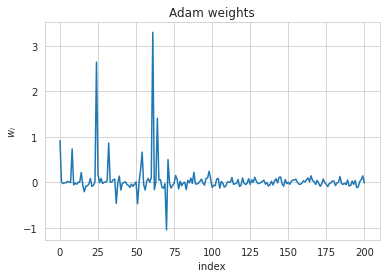
To test how these solutions generalize, we can imagine partitioning the dataset into a train and test split. Because of how we’ve constructed the data, naively taking the features from the original problem will be a less informative experiment than one might initially expect. Several indices of the features will be zero for all training inputs, meaning that there is no gradient for the optimizer to reduce whatever initial weight was assigned to these indices, and so both GD and adam should generalize similarly based on their initialization. If we add a small amount of noise to the features, so that we define each data point \(\boldsymbol{x}_i, i=1\dots n\) as \(e_i + y_i e_{n+1} + \epsilon_{i}\), where \(y_i \sim \mathcal{N}(0, 1)\), with \(\epsilon_{i} \in \mathbb{R}^{n+1} \sim \epsilon \mathcal{N}(0, Id)\) for some small but nonzero \(\epsilon\), then the zero-gradients issue goes away while preserving the intuition of the original problem setting that one feature is significantly more predictive of the outcome than any other.

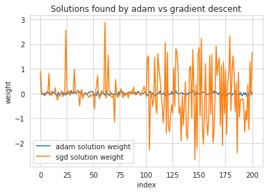
After training with gradient descent and adam, we essentially replicate the result above: gradient descent assigns a high magnitude to the generalizing feature and low magnitudes to the rest. Adam assigns large magnitudes all over the place. However, adam converges faster and gets lower training error after a truncated training period of 1000 steps. We might be a bit conflicted then on which solution we should pick – in previous papers I did suggest that training speed should be indicative of generalization in at least some cases. To give some hint as to which way the answer to this question will go, I present without further comment the weights learned by adam and sgd on this problem.

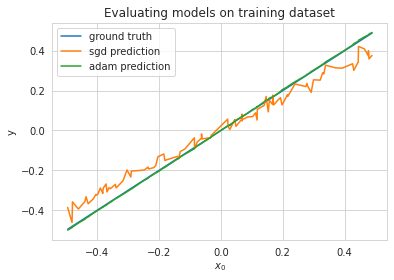
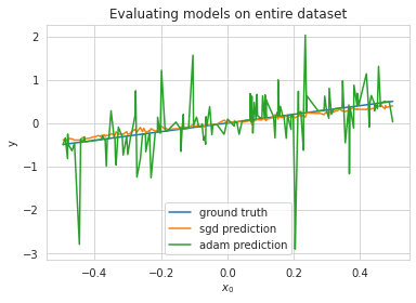
To evaluate how well the two solutions generalize, I looked at what happened when training on 100 points of a 200-datapoint dataset and then evaluating both SGD and Adam on the entire set of points. The result is as would be expected: while adam is perfectly able to fit its training set, the high weight magnitude to somewhat random indices elsewhere contribute to gigantic errors on the test points.

Obviously, this setting is a bit contrived. For starters, it will be extremely rare in naturally occuring data for the principal component to be precisely axis-aligned with a single parameter. Adam’s second-moment correction is axis-aligned, and so the situation constructed in this blog post is probably the absolute worst-case setting you could put adam into. I tried replicating the analysis described in this blog post with non-axis-aligned features, and the result was much closer to what is reported in practice: gradient descent exhibited slightly better generalization, but nothing crazy like in the example here. Generally speaking, while it seems like adaptive learning rates have the potential to catastrophically affect generalization, in practice they don’t because they’re not very good at approximating curvature when features aren’t axis-aligned.