What's grokking good for?

Some intuition on the what, why, and how of delayed generalization

A primer on delayed generalization

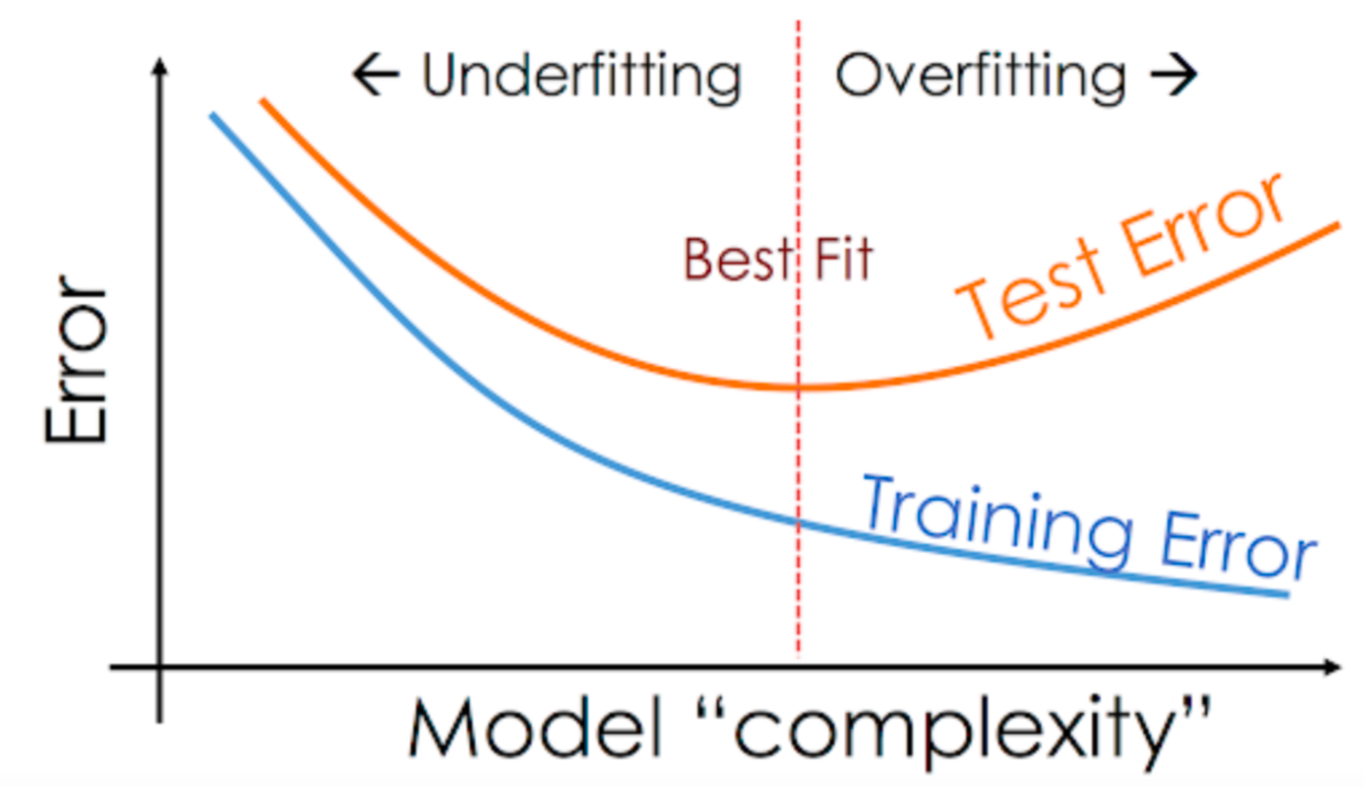
The traditional school of machine learning theory states that as your model class becomes more complex, you should expect whatever function your training algorithm finds in that model class to fit your training dataset will be worse, on average, at generalizing to new data. One passes neatly between three regimes: from under-fitting to fitting to over-fitting. Machine learning textbooks in 2017, when I was in school, particularly loved the following visualization.

The justification for this figure is based on decades of beautiful work in statistical learning theory. For a brief primer, you can refer to earlier posts on e.g. PAC-Bayesian generalization bounds or model complexity measures for modern machine learning. The mathematics underlying the relationship between the empirical and expected risk are deep. They also utterly fail to predict the behaviour of modern deep learning systems.

At first glance, this received wisdom isn’t completely at odds with the modern era of “jUsT aDd MorE LaYerS BrO” because typically when we add more layers we also add more data. But the past five years have shown that even in more rigorous evaluations, the traditional maxim of “bigger model, worse generalization” fails to hold. In particular, a phenomenon known as double (or even multiple) descent has emerged, whereby the previous figure is replaced by the following one.

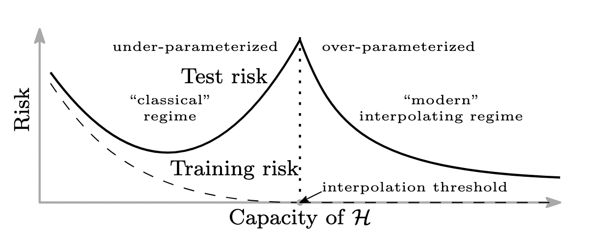
In short: deep learning systems behave qualitatively as predicted by statistical learning theory up until the point where they can perfectly fit their training data. At this point, generalization performance tends to improve. This can be loosely thought of as happening because neural network training has a number of properties that bias it towards functions that generalize well. As the model capacity gets bigger, there are more functions to choose from which fit the training data and the generalization performance increases. Bringing the model closer to the threshold where it can just barely interpolate its training data, whether that is by reducing training time, expanding the data set, or decreasing model size, hurts performance. In the case of training time, double descent can also be referred to as ‘delayed generalization’, as we see generalization increase later in time as the model has trained for longer.

Grokking

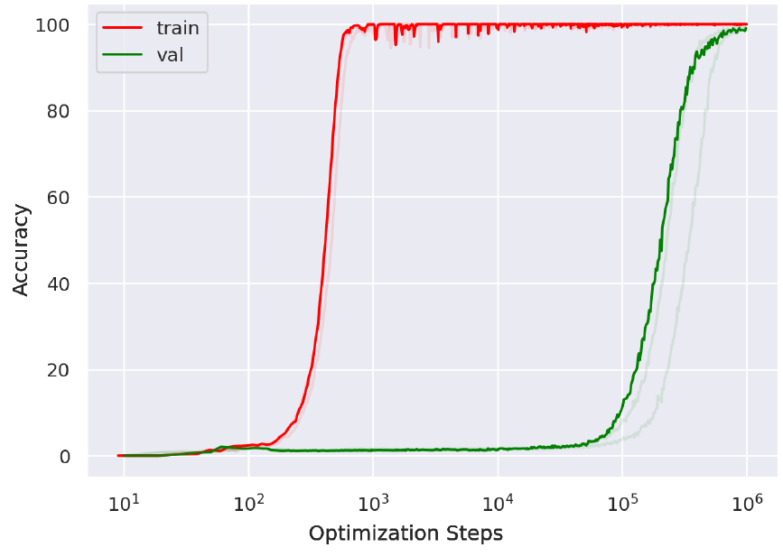
There is a third regime of generalization, which has been observed primarily but not exclusively in transformers trained on mathematical datasets, in which rather than gradually seeing smooth improvements in generalization as the model class complexity grows (e.g. as training time increases), generalization occurs relatively suddenly and after a long period of zero generalization. This phenomenon, while it falls loosely under the bucket of ‘delayed generalization’, is known as grokking.

Thanks in part to its catchy name and in part due to its mysterious nature and potential implications for emergent capabilities in more capable systems, grokking has captured the attention of the AI Safety and Mechanistic Interpretability communities. I understand the appeal: when a network groks, we see no change in its behaviour on the training set while it “secretly” develops a deeper level of reasoning.

At this point, grokking is very well understood. We now have progress measures as well as several model systems where it can be induced, including MNIST. We have several methods for accelerating grokking, and several only-slightly-contradictory explanations for why it occurs. In a surprising win for deep learning theory research, analytical work studying the learning dynamics of infinite-width neural networks has actually been useful in providing a spiritual framework, if not precisely a concrete mathematical characterization, for understanding what is happening in neural networks when they grok.

Grokking as feature-learning

The model that people have converged on in recent years is that grokking is essentially a natural consequence of the same underlying forces that drive delayed generalization and double descent. Neural network optimization has a bias towards functions that generalize well, but it can take a while for this bias to materialize during optimization if, for example, the network is initialized in a regime where there are many local minima that do not generalize well. In this case, it is vanishingly unlikely that the first local minimum the network finds will be a good one.

Ending up in a bad local minimum is bad for optimization because it means you don’t have much gradient signal to work with, and optimization will take small steps. Small steps mean that any inductive bias given by the optimization process will take a long time to show up in your function, because it takes a long time for the optimizer to make meaningful changes to the parameters. These underlying dynamics are largely to blame for the slow emergence of generalization in networks that grok, and why grokking hadn’t been seen in e.g. computer vision tasks. Vision tasks use architectures with such a strong inductive bias that even random sampling of parameters tends not to overfit. Without an abundance of bad minima near the initial parameters, optimizers tend not to immediately converge to a bad local minimum and we see smoother generalization performance. In works that have managed to induce grokking in vision tasks, bizarre initializations have to be constructed so that the loss landscape does have “bad” (although not as “bad” as in modular arithmetic tasks) local minima that could attract gradient-based optimizers at initialization.

Transformers, being as close as we can get to a blank slate in a neural network architecture, are much more vulnerable to poorly-generalizing local minima. Modular arithmetic is also a relatively pure task: whereas in most natural datasets the network must learn a huge variety of relationships between inputs and outputs and this immense diversity allows for smooth behaviour as subtasks “average out”, adding two numbers together doesn’t decompose naturally into sub-skills. Performance is going to be relatively binary in this case compared to, say, translating texts or answering LSAT problems. In the latter case, even if the task can be composed into a collection of sub-tasks with binary performance, there are enough subtasks that the resulting learning curves look smooth to a human observer.

So, we have a sense of why there would be a gap between interpolation and generalization, and why it’s reasonable to expect a fairly rapid transition to a generalizing solution. What’s missing is still a question of how networks find this generalizing solution. Surely, I can hear you say, it’s not a matter of waving a magical “implicit bias of gradient-based optimization” wand and waiting? While I would be overjoyed for such a wand to exist, you would be correct. Instead of a magic wand, it’s perhaps easier to think of gradient descent as a kind of dynamical process, which tends to converge to certain types of minima as a result of the pressures put on the network by the optimizer dynamics.

The exact mechanics underlying the transition from memorization to generalization will differ a bit from task to task, but the overall picture goes something as follows: the network starts out with some initial features, and with a very minor change to its parameters is able to use those features to reach ~0 train loss (this is known as the “lazy” regime). While at ~0 train loss, weight decay is providing a slight pressure on the model to reduce its parameter norm, and this pressure is the main driving force that allows the network to make small but nonzero changes to the learned features. In particular, every optimizer step is slightly shrinking the parameters and applying a small perturbation that is hopefully in the direction of reducing the training loss. At equilibrium, these two forces cancel out, and the network looks like it has hit a stable plateau of ~constant parameter norm and ~constant loss.

Under the surface, however, each step of gradient descent is a battle. Weight decay shrinks the parameters towards zero, and the gradient fights back by pushing the parameters back in the direction that moves the loss down as quickly as possible. Unless the network is already at a min-norm solution, the gradient step won’t exactly reinforce the current parameters — instead, this process will reinforce the sub-networks that give the best nats-per-parameter-norm, and slowly decay away the sub-networks that don’t. Using a higher value of weight decay or a higher learning rate will make the steps taken in this equilibrium phase larger, allowing it to happen faster, and amplifying the low-frequency components of the updates will also more rapidly facilitate this process. However this occurs, eventually, once this best-value circuit is sufficiently amplified, the winner-take-all dynamics of neural networks will lead to its fairly rapid adoption. This phase is easy to identify because the parameter norm suddenly drops and test accuracy goes to 100%. It is also the cause for some confusion about whether grokking happens because the parameter norm is small, or whether parameter norm drops because grokking happens. I lean more towards the latter, but will dive into this more in a follow-up post.

A great deal of work on mechanistic interpretability tries to understand the properties of the generalizing solution once it has been found. For example, some works have visualized the features of mod p arithmetic problems as encoding a cyclic relationship between numbers. Others have tried to reconstruct the algorithm encoded by the network. This type of result is extremely impressive and requires painstaking analysis of the netural network weights and features. The inferential leaps required to uncover even the circuits underlying addition make me skeptical of the feasibility of this type of decomposition for more complex tasks. Instead of understanding what the network learns, I think that studying grokking is interesting for a different reason: understanding how neural networks are able to overwrite “bad” features and replace them with better ones.

Is understanding grokking even worth it?

In the face of the abundant literature on grokking, a question arises: what’s all of this research for? Why are taxpayer dollars funding research on neural networks learning to add numbers together in this era of LLMs?

The early justification for studying grokking was that it presented a phase transition in network capabilities which, while not particularly concerning for basic math skills, suggested that perhaps more dangerous capabilities might suddenly arrive without warning in larger models. Understanding how these capabilities emerge and whether they can be detected in advance would be useful for frontier labs monitoring their training runs for emergent dangerous capabilities. And yet I think the past few years’ study of grokking has also revealed that it is a fruitful testbed for answering basic questions about neural network learning dynamics.

The success of scaling laws can in large part be attributed to the immense scale at which we train current systems. Although natural language datasets are fundamentally discrete, they are made up of so many fundamental discrete bits that when you squint at them they look virtually continuous. This continuity means that even if we can’t say precisely which discrete capabilities the network will extract from its training data at any given time, we can be roughly sure that whatever it learned will map reliably onto a small range of predictive log likelihood. Grokking occurs when there is only one thing (or at best a small handful of things) to learn, and the dataset is small enough that it is quickly exhausted. It provides hope that, even if we run out of human data, the right type of inductive bias might allow training algorithms to continue to improve performance by searching for increasingly simple and powerful explanations of the training data.

This type of learning is reminiscent of the process of science, seeking increasingly fundamental explanations for the universe. It is also still something that, at least in deep learning systems, is poorly understood. How do we induce the right kind of dynamics to facilitate simplicity bias without underfitting? How do we know whether a network has learned everything it can from a particular dataset? These questions remain fundamental open problems, and answering them would take us into a new regime of neural network training where, rather than passively hoping that networks extract the information from the data stream that will translate to useful and general capabilities, we are able to take a more active role in steering training dynamics.

In my next blog post (which will hopefully come out soon once I finally post the paper on arxiv) I’ll lay out my attempt at addressing these questions, which I’ll also be presenting at CoLLAs and would be happy to chat about with folks who will be there!